


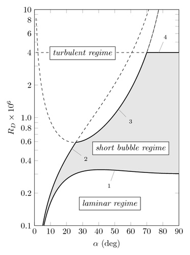
This is one I like from my thesis. It illustrates the predicted boundaries for boundary layer transition mechanisms on a cylindrical afterbody at incidence:
- free shear-layer instability,
- ttachment-line instability,
- cross-flow instability,
- streamwise-flow instability.
\documentclass[border=5pt]{standalone}
\usepackage{pgfplots}
\pgfplotsset{width=7cm,compat=1.8}
%% free shear-layer instability (fsli)
\pgfmathdeclarefunction{fsli}{1}{%
  \pgfmathparse{ tan(#1)/( cos(#1)*( 1 + 3.3*((tan(#1))^2) ) ) }%
}%
%
%% attachment-line instability (ali)
\pgfmathdeclarefunction{ali}{1}{%
  \pgfmathparse{ 1.1*tan(#1)*(1/cos(#1)) }%
}%
%
%% cross-flow instability (csi)
\pgfmathdeclarefunction{csi}{1}{%
  \pgfmathparse{ 0.145*( ( 1 + 3.3*(tan(#1))^2 ) / sin(#1) ) }%
}%
%
%% streamwise-flow instability (sfi)
\pgfmathdeclarefunction{sfi}{1}{%
  \pgfmathparse{ 4 }%
}%
%
%% piecewise function (combining ali, csi and sfi)
\pgfmathdeclarefunction{alicsisfi}{1}{%
  \pgfmathparse{%
    (and( #1>=1    , #1<=25.78) * ( ali(x) ) +%
    (and( #1>25.78 , #1<=70.00) * ( csi(x) ) +%
                (and( #1>70.00 , #1<=89.99) * ( sfi(x) )  %
   }%
}%
\begin{document}
\begin{tikzpicture}

% set style options for annotations with pins (see bottom of tikzpicture)
\tikzset{%
   every pin/.style={draw=none,
                     fill=none,
                     %rectangle,rounded corners=0pt,
                     font=\scriptsize}
                 }

\begin{semilogyaxis}[%
  %
  view={0}{90},
  width=0.50\linewidth,height=0.75\linewidth,
  %
  scale only axis,
  axis on top=false,
  axis lines*=box,
  %
  xmin=0, xmax=90,
  xtick={0,10,20,30,40,50,60,70,80,90},
  xlabel={\raisebox{0pt}[\height][\depth]{$\alpha$ (deg)}},
  %
  ymin=0.1, ymax=10,
  ytick={0.1,0.2,0.3,0.4,0.5,0.6,0.7,0.8,0.9,1.0,2,3,4,5,6,7,8,9,10},
  yticklabels={0.1,0.2,{},0.4,{},0.6,{},0.8,{},1.0,2,{},4,{},6,{},8,{},10},
  ylabel={\raisebox{0pt}[\height][\depth]{$R_D \times 10^{6}$}},
]

%% fsli (start stacking)
\addplot[
  domain=1:89.99,samples=225,
  draw=none,fill=none,mark=none,
  stack plots=y]
  { fsli(x) };
%
%% stack difference between alicsisfi (upper) and fsli (lower) curves on top of fsli and fill area
\addplot[
  domain=1:89.99,samples=225,
  draw=none,
  fill=black!10,
  stack plots=y]
  { max( alicsisfi(x) - fsli(x) , 0 ) } % area above fsli and below alicsisfi
  \closedcycle;

%% fsli, alpha = [1 , 89.99]
\addplot[
  domain=1:89.99,samples=225,
  solid,line width=0.8pt,draw=black,mark=none]
  { fsli(x) };

%% ali (1), alpha = [1 , 25.78]
\addplot[
  domain=1:25.78,samples=62,
  solid,line width=0.8pt,draw=black,mark=none]
  { ali(x) };
%
%% ali (2), alpha = [25.78 , 89.99]
\addplot[
  domain=25.78:89.99,samples=163,
  dashed,draw=black,mark=none]
  { ali(x) };

%% csi (1), alpha = [1 , 25.78]
\addplot[
  domain=1:89.99,samples=62,
  dashed,draw=black,mark=none]
  { csi(x) };
%
%% csi (2), alpha = [25.78 , 70]
\addplot[
  domain=25.78:70,samples=112,
  solid,line width=0.8pt,draw=black,mark=none]
  { csi(x) };
%
%% csi (3), alpha = [70 , 89.99]
\addplot[
  domain=70:89.99,samples=174,
  dashed,draw=black,mark=none]
  { csi(x) };

%% sfi (1), alpha = [1 , 70]
\addplot[
  domain=1:70,samples=350,
  dashed,draw=black,mark=none]
  { sfi(x) };
%
%% sfi (2), alpha = [70 , 89.99]
\addplot[
  domain=70:89.99,samples=51,
  solid,line width=0.8pt,draw=black,mark=none]
  { sfi(x) };

%% annotations (see style options for pins set with \tikzset above)
\node[coordinate,pin=-95:{1}] at (axis cs:50,0.326) {};
\node[coordinate,pin=-30:{2}] at (axis cs:23.3,0.5158) {};
\node[coordinate,pin=below right:{3}] at (axis cs:52.3,1.196) {};
\node[coordinate,pin=80:{4}] at (axis cs:77.5,4) {};
%
\node[draw=black,fill=white] at (axis cs:47,0.16) {\emph{laminar regime}};
\node[draw=black,fill=white] at (axis cs:60,0.52) {\emph{short bubble regime}};
\node[draw=black,fill=white] at (axis cs:30,3.95) {\emph{turbulent regime}};

\end{semilogyaxis}
\end{tikzpicture}
\end{document}