


That’s from my German blog TikZ.de.
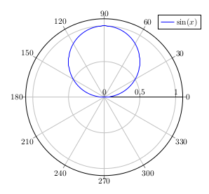
Recently I played with the sine function, that “wave” that everybody knows in cartesian coordinates. Let’s take a look at a 3d polar complex sine made plot.
In polar coordinates the sine function is a simple circle:
\documentclass[border=10pt]{standalone}
\usepackage{pgfplots}
\usepgfplotslibrary{polar}
\begin{document}
\begin{tikzpicture}
  \begin{polaraxis}[
      domain  = 0:180,
      samples = 100,
    ]
    \addplot[thick, blue] {sin(x)};
    \legend{$\sin(x)$}
	\end{polaraxis}
\end{tikzpicture}
\end{document}
When we shorten the period length, we get:
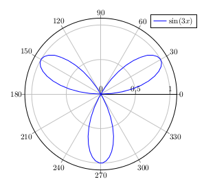
We can take a rational factor:
\documentclass{standalone}
\usepackage{pgfplots}
\usepgfplotslibrary{polar,colormaps}
\begin{document}
\begin{tikzpicture}
  \begin{polaraxis}[
      domain  = -14400:14400,
      samples = 3000,
      colormap/cool,
      hide axis
    ]
    \addplot[no markers,mesh,opacity=0.5] {1-sin(40*x/39};
  \end{polaraxis}
\end{tikzpicture}
\end{document}
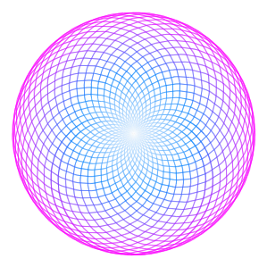
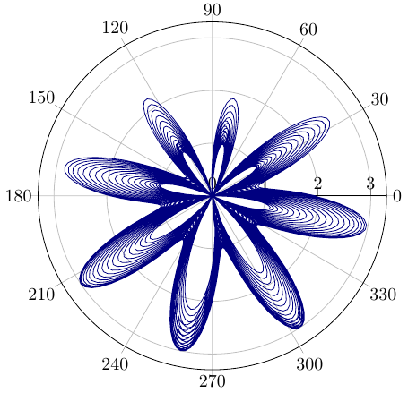
By adding another sine with other factors, we get more movement:
\documentclass{standalone}
\usepackage{pgfplots}
\usepgfplotslibrary{polar}
\begin{document}
\begin{tikzpicture}
  \begin{polaraxis}[
      domain = -3600:3600,
      samples = 4000
    ]
    \addplot[blue!50!black] {1 - sin(50*x/49) - sin(8*x)};
  \end{polaraxis}
\end{tikzpicture}
\end{document}
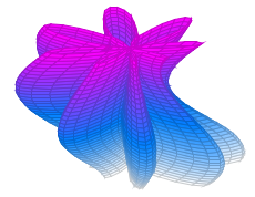
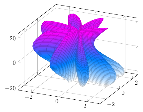
Let’s have a 3d view with growing angle.
We make a parametrical 3d-Plot in x and y: x runs the circle from -180 to 180 degree, we make a sampling for y for the number of rotations. We add y time 360 degrees to the function argument. y is our third dimension, while x as angle and the function value are the the original two dimensions.
\documentclass[border=10pt]{standalone}
\usepackage{pgfplots}
\begin{document}
\begin{tikzpicture}
  \begin{axis}[
      domain    = -180:180,
      y domain  = -19:19,
      samples y = 39,
      samples   = 100,
      z buffer  = sort,
      colormap/cool,
      grid
    ]
    \addplot3[data cs = polar, surf]
      ( {x}, {1 - sin(50*(x+360*y)/49) - sin(8*(x+360*y))}, {y} );
    \end{axis}
\end{tikzpicture}
\end{document}
That was my todays voyage from a circle to a rather complex function in 3d.